
Jump to commodity and equity sensitivity tables →
Merton v2: research and decisions
Update: Merton 2.2 replaces the box Robust objective with mean scenario utility minus portfolio-level forecast dispersion, adds sensitivity tables, and strengthens publication consistency. See v2.2 decisions. The original v2.0 findings below remain a historical record.
Update: Merton 2.1 replaces the VTIP three/seven-year return blend. The tables below document the original 2.0 research snapshot. See the VTIP correction and purchasing-power research.
Research cutoff: October 2, 2026 (completed Friday observations). Portfolio example: October 5 market inputs, reviewed October 6. These are conditional research allocations, not personalized advice.
Decision
Use ten-year geometric CAGR forecasts, convert them to continuous Merton drift, and publish both Central and Robust allocations. Retain the configurable 20% BTC and 7% gold priors. Neither is an empirically established expected return. Gold’s historical ten-year median CAGR in this sample was only 3.4%, so 7% is an optimistic structural judgment.
The BTC terminal-multiple experiment is promising, but does not yet justify a ten-year production forecast. Gold’s 200WMA models did not improve out-of-sample forecasts. No moving-average signal, KISS filter, market-timing rule or required diversification allocation enters v2.
The pre-change audit records the original implementation. The protocol was recorded before fitting. Full numeric artifacts accompany this report: forecast results, research diagnostics, portfolio sensitivity, portfolio scenarios and source manifest.
1. The old return interpretation was wrong for the intended priors
The existing solver maximizes wᵀ(μ − r1) − γ wᵀΣw / 2. It uses diffusion drift, annualized log-return covariance, long-only weights, no borrowing, six optional caps, residual cash and γ=3. Its exact active-set optimization remains appropriate. This is the constrained strategic allocation part of Merton, not his entire consumption/lifecycle problem. Stanford Merton lecture.
For dS/S = μ dt + σ dW, log growth is μ − σ²/2. Therefore:
- Input geometric CAGR
g = exp(μ − σ²/2) − 1. - Merton drift
μ = ln(1 + g) + σ²/2. - One-year simple arithmetic expected return
E[S₁/S₀ − 1] = exp(μ) − 1.
The optimizer requires the second quantity, not the third. The relationship is exact under its constant-parameter geometric Brownian motion assumption. Portfolio CAGR uses portfolio drift minus half portfolio variance, not a weighted average of individual CAGRs.
| Assumption | Volatility | Required Merton drift | One-year simple arithmetic expectation |
|---|---|---|---|
| BTC 20% CAGR | 60.0% | 36.23% | 43.67% |
| Gold 7% CAGR | 19.52% current risk estimate | 8.67% | 9.06% |
| Gold 7% CAGR | 20.0% illustrative | 8.77% | 9.16% |
Old BTC μ=20% implied only 2.02% geometric growth at 60% volatility. Old gold μ=7% implied 5.23% at the current volatility. This corrects a units error; it does not validate either structural forecast.
The candidate sqrt((1+g)²+σ²)−1 is exact for the geometric mean of two equally probable simple returns a±σ, since (1+g)²=(1+a)²−σ². That is a different return distribution and a different volatility definition. It gives BTC approximately 34.16%, which is neither the required diffusion drift nor the GBM one-year arithmetic expectation. Using it here would mix conventions.
“Expected CAGR” means model-implied geometric growth. It is not literally the expectation of the random finite-horizon CAGR: under GBM that expectation is exp(μ−σ²/2+σ²/(2H))−1. This distinction matters for high volatility and short horizons. A ten-year strategic forecast is not a claim that realized annual returns are Gaussian, stationary or predictable.
2. A common ten-year horizon
| Asset | Ten-year CAGR method | Example CAGR | Main uncertainty |
|---|---|---|---|
| SPY | Dividend flow + 5% nominal per-share EPS growth + normalization from FY1 P/E 20.72 to 18 over ten years, less fee; exponentiate log growth | 4.57% | Growth, terminal valuation, dividend approximation |
| IEF | Starting YTM less fund fee | 5.12% | Rolling duration 6.85 and maturity 8.45 years differ from ten-year horizon; reinvestment, roll and repricing |
| VTIP | Three years of initial net real carry plus ten-year inflation compensation; seven years at strategic gross short rate less VTIP fee; blend in log units | 4.37% | Turnover assumption, future real yields, inflation compensation and reinvestment |
| GLDM | Configurable net structural prior | 7.00% | No dependable cash-flow valuation |
| PDBC | Strategic gross cash collateral rate + selected 2% continuous futures premium − fund fee, exponentiated | 5.74% | Spot/roll premium, collateral implementation and future fees |
| FBTC | Configurable net structural prior | 20.00% | Adoption, competition, regulation, permanent loss and changing market structure |
| SPAXX | Ten-year expected average short rate from Fed Kim–Wright, less fund fee, exponentiated | 3.82% | Term-structure model, future policy and fees |
Equity growth includes inflation and buybacks; neither is added twice. Bond YTM is a practical anchor, not a guaranteed ETF return. We do not add a speculative roll-down return on top. Vanguard on starting bond yields and investment horizons.
The cash anchor is the Fed model’s ten-year zero yield less its term premium: 5.2551% − 1.0847% = 4.1704%, continuously compounded. Subtracting SPAXX’s 0.42% fee gives expm1(3.7504%) = 3.82%. Raw forward rates contain risk premiums; they are not automatically expected policy rates. The Fed model is survey-informed, revisable and uncertain. Its weekly source gets an eight-weekday expiry. Fed Kim–Wright methodology, Fidelity expense disclosure.
VTIP’s net SEC yield explicitly excludes inflation indexation. The ten-year inflation-compensation estimate is 2.3334% in continuous units. We combine ln(1+net real SEC yield) with that compensation; no second fee is deducted from the already-net initial yield. The later reinvestment anchor deducts VTIP’s 0.03% fee once. The three/seven-year bridge is a transparent strategic assumption, not a backtested optimum or a promised maturity payoff. The source yield is a carry proxy, and the unit transformation does not make it an exact holding-period return. Fed TIPS curve, Vanguard yield convention, VTIP prospectus fee.
3. What the 200WMA experiments actually found
BTC uses Coin Metrics daily USD prices from July 2010; gold uses World Gold Council daily USD spot prices from the floating-price era beginning August 1971. We select the final close of each completed Friday week, require 200 consecutive weeks, and calculate price/200WMA plus annualized 13-, 26- and 52-week MA growth and a 52-week log-MA regression slope. Gold is collected in annual windows because the provider thins long chart requests. Raw licensed prices are cached locally, not redistributed. Coin Metrics community data, World Gold Council prices.
Forward labels end at the first weekly close on/after the calendar anniversary and annualize actual elapsed days. At every origin, training labels must have ended strictly before that origin. At least 104 matured training observations are required. These are overlapping weeks, not 104 independent returns. Every model at a horizon uses the same test origins. We do not clip bad forecasts to improve errors.
Benchmarks include constant priors, expanding historical mean, four slope variants, extension only, each slope plus extension, a fixed 50/50 blend of the prior and 52-week combined regression, and terminal-multiple models. Terminal multiples are expanding historical medians observed by the forecast date, not full-sample medians. One terminal model grows the MA at its current slope; the other uses the structural prior. Coefficients, forecast correlations, direction calibration, subperiods, block intervals and nonoverlapping-offset checks are in the diagnostics.
| Asset / horizon | Fixed prior RMSE | Slope 52w | Extension | Combined 52w | 50/50 blend | Terminal + prior | Weekly forecasts / full horizon blocks |
|---|---|---|---|---|---|---|---|
| BTC 1y | 158.0 | 504.9 | 261.3 | 430.1 | 233.6 | 141.9 | 385 / 7 |
| BTC 3y | 27.7 | 81.7 | 88.7 | 87.2 | 35.5 | 13.7 | 177 / 1 |
| Gold 1y | 19.9 | 32.8 | 36.8 | 43.4 | 28.4 | 33.2 | 2,416 / 45 |
| Gold 3y | 11.3 | 21.1 | 21.9 | 23.2 | 15.8 | 14.8 | 2,208 / 14 |
| Gold 5y | 9.1 | 13.1 | 13.7 | 14.3 | 11.3 | 10.9 | 2,000 / 7 |
| Gold 10y | 6.7 | 9.6 | 9.9 | 10.3 | 8.2 | 6.9 | 1,478 / 2 |
RMSE is percentage points of realized CAGR. BTC five-year testing has no out-of-sample observations after the declared feature/training/label requirements; claiming a five-year validation would be misleading. Gold ten-year tests also have fewer than three full test horizons.
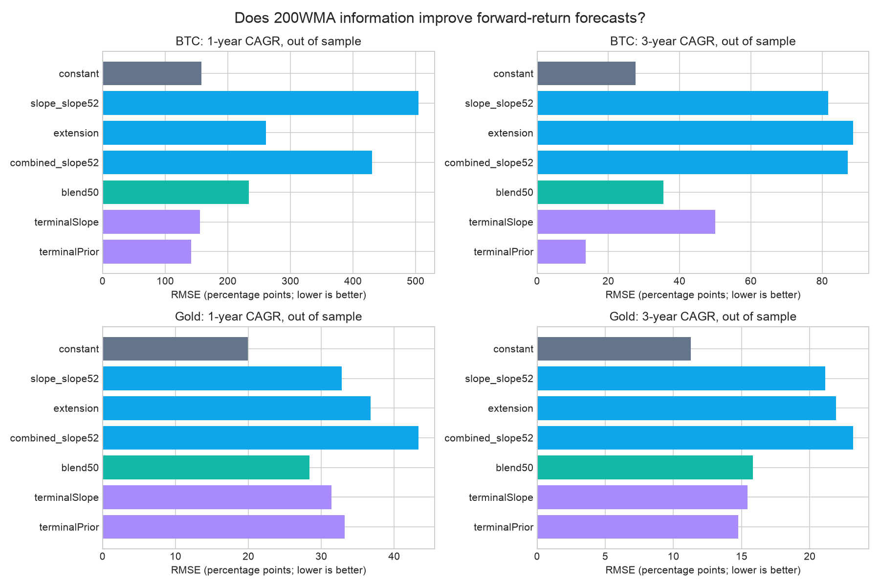
BTC slope does not show a stable positive relationship: combined-model slope coefficients are −0.65, +0.14 and −0.16 for one/three/five-year in-sample fits. Extension coefficients are negative (−0.41, −0.46, −0.40), with stronger in-sample three/five-year evidence. However, regressions extrapolate poorly out of sample. A high forecast correlation does not rescue a badly biased level forecast. Gold’s one-year slope is negative and extension positive, contrary to the proposed signs; neither gives a useful stable production rule.
BTC’s terminal-prior result deserves follow-up. Its one-year squared-error improvement also survives the chosen 90% horizon-block bootstrap (loss difference interval −0.97 to −0.08 in squared CAGR units), conditional on this sample and protocol. It improves one-year RMSE in both test halves, but its three-year advantage occurs mostly in the second half (first half RMSE 14.8 vs prior 14.6 pp; second half 12.5 vs 36.2 pp). One overlapping three-year cycle cannot establish a ten-year forecast model. Promoting whichever tested variant wins would also introduce model-selection bias. The 20% prior was selected in 2026: these are retrospective benchmark comparisons, not evidence that an investor specified it in 2010.
Historical BTC extension P10/median/P90 is 1.02× / 1.80× / 4.32×. Five-year-era medians decline from about 3.01× in early available history to 1.92× in 2015–19 and 1.62× in 2020–24. Gold’s corresponding distribution is 0.84× / 1.07× / 1.47× and also varies across regimes. Neither a 1.0 multiple nor the full-sample median is a proven fair value.
Single-risky-asset/cash economic diagnostics use γ=3, fixed volatility, weekly rebalancing and no costs. They are available in results.json as a limited forecast-sizing check, not a historical multi-asset v2 track record. Reconstructing dated equity forecasts, term-premium vintages, fund availability and covariance at each historical date would be required for such a claim. Revised source histories and survivorship remain limitations.
4. Uncertainty and the Robust objective
We use triangular CAGR distributions with explicit lower support, base-case mode and upper support. They express judgment about the expected mean, not annual return shocks or statistical confidence bounds.
| Asset | Lower / base / upper CAGR |
|---|---|
| BTC | −10% / 20% / 50% |
| Gold | −3% / 7% / 15% |
| SPY | Base ±3 percentage points |
| IEF, VTIP, cash | Base ±1.5 percentage points |
| PDBC | Base ±4 percentage points |
The proposed BTC 10–30% and gold 3–10% bands exclude plausible weak long-run outcomes. We broaden them deliberately. Gold’s observed ten-year P10/median/P90 is approximately −3.1% / 3.4% / 14.2%; that motivates adverse scenarios but is not an estimate of uncertainty in today’s mean. BTC’s limited, nonstationary history cannot calibrate a ten-year mean confidence interval. The BTC band includes negative growth but not total failure; permanent loss requires a separate stress, and no finite diffusion volatility represents it faithfully.
For 8,192 seeded draws, convert each CAGR to μ and solve the constrained portfolio with fixed return covariance. Compute δᵢ = SD(μᵢ − r) across the draws, including cash forecast uncertainty. Robust Merton solves:
max_w wᵀ(μcentral − rcentral) − γ wᵀΣw/2 − Σᵢ wᵢ δᵢ.
This is exact max–min optimization over the rectangular ambiguity set eᵢ ∈ [ecentralᵢ−δᵢ, ecentralᵢ+δᵢ], since all weights are nonnegative. The penalty strength is one, an explicit conservative preference, not a fitted statistical confidence level. Box uncertainty allows all risky excess means to disappoint together and can be more conservative than an ellipsoid. It is understandable, reproducible and uses the already independently verified quadratic solver. Robust portfolio selection research.
Averaging scenario-optimal weights has no equivalent objective here. Maximizing expected quadratic utility over uncertain means with fixed Σ merely substitutes the mean μ and introduces no uncertainty penalty. We therefore use the explicit worst-case criterion. Return covariance is not randomly perturbed: that would add another difficult-to-calibrate distribution. Separate volatility stresses are reported instead.
5. How much allocations depend on assumptions
| Asset | Central γ=3 | Robust γ=3 | Scenario P10 | Median | P90 |
|---|---|---|---|---|---|
| SPY | 0% | 0% | 0% | 0% | 4% |
| IEF | 35% | 53% | 0% | 28% | 56% |
| VTIP | 0% | 0% | 0% | 0% | 22% |
| Gold | 19% | 0% | 0% | 14% | 55% |
| PDBC | 17% | 17% | 0% | 14% | 35% |
| BTC | 28% | 20% | 14% | 28% | 40% |
| Cash | 0% | 10% | 0% | 0% | 0% |
Marginal quantiles are not a feasible portfolio and need not sum to 100%. Robust cash can exceed the simulated optimal cash quantile because its simultaneous adverse excess means differ from typical independent draws. Gold’s zero Robust weight is a consequence of its uncertain excess mean, not a claim that gold has no role for every investor.
The independent alternate seed changes the largest displayed quantile by about 0.5 pp; split-half estimates differ by up to 2.6 pp. Numerical quantiles are approximate, especially where allocations change boundary. We display whole percentage weights, keep the seed public, and do not imply sub-percentage certainty.
| γ | Central BTC | Robust BTC | Robust cash |
|---|---|---|---|
| 1 | 81% | 59% | 0% |
| 2 | 42% | 30% | 0% |
| 3 | 28% | 20% | 10% |
| 4 | 21% | 15% | 32% |
| 6 | 14% | 10% | 55% |
| 10 | 9% | 6% | 73% |
γ is investor risk preference, not a forecast. No evidence here justifies changing the default of three. Low γ exposes how aggressive the corrected BTC prior can be. Full asset tables, BTC/gold low/base/high scenarios and volatility stresses are in the linked portfolio artifacts.
6. VTIP and remaining risks
VTIP’s adjusted daily log-return volatility since October 2012 is 2.52%; rolling one-year P10/median/P90 is 1.40% / 1.92% / 4.24%. Calendar-year volatility reached about 5.14% in 2020 and 4.30% in 2022. Thus the existing 3% floor is defensible for ordinary conditions but understates stress regimes. A large optimizer weight can result from a small, overly certain excess-return assumption, not necessarily a bad measured volatility.
We retain the floor, expose a 5% VTIP stress, and address reinvestment and mean uncertainty directly. We do not impose an arbitrary VTIP cap to obtain a desired allocation. At the reference inputs it receives zero centrally but up to roughly 22% at P90 across forecasts, demonstrating continued assumption sensitivity.
The original risk estimator remains: equal blend of ten-year proxy and available actual ETF covariance, aligned daily log returns annualized by 252, 20% correlation shrinkage toward independence and floors of 18/7/3/18/18/60%. Gold and BTC proxies extend their short ETF histories. ETF/spot close times differ; BTC trades weekends and can jump. Current risk estimates are not point-in-time historical estimates for the forecasting experiment.
Largest limitations: judgmental central means and scenario supports; independent forecast draws despite shared inflation/policy risks; no joint probability interpretation for the Robust box; revised term-structure estimates; no long BTC validation horizon; gold regime shifts; fees and rolling-bond behavior; static covariance; fixed geometric growth making required μ increase with assumed variance; no taxes, slippage, investor liabilities or consumption model. The model may be wrong in ways outside every displayed scenario.
Reproduction and verification
Create a Python environment and install scripts/merton-v2-requirements.txt. Run:
python scripts/collect-merton-v2-research.py
python scripts/analyze-merton-v2.py
python scripts/test-merton-research.py
python scripts/verify-merton-v2-scipy.py
node scripts/analyze-merton-v2-portfolios.mjs
npm run test:merton
The manifest records public source URLs, retrieval times, hashes and failures. Raw data stay in ignored .cache/merton-v2/. FRED direct downloads failed; the implemented strategic rate/inflation inputs use the Federal Reserve’s own fitted-curve CSVs. Source revisions mean a future re-download can differ; retaining the cached hashes allows an audit of this run.
Tests cover exact conversion examples, invalid domains, analytic robust solutions, cash/cap/no-leverage boundaries, fixed-seed simulation, corrupted feed rejection, 24 independent SciPy v2 portfolio cases plus the 42 existing solver fixtures, weekly MA/slope/extension calculations and calendar labels. Future-price perturbation and prefix truncation leave past forecasts unchanged. Historical v1 publications remain readable with their original return convention; v2 is an explicit contract/methodology upgrade.
Merton v2.2: validation and decisions
Research completed October 6, 2026. The tables in this section use the frozen v2.1 market inputs so methodology effects are isolated from subsequent market changes. Production refreshes those inputs. Reproduce with scripts/analyze-merton-v22.py in the pinned research environment; all scenario results and full comparison tables include every asset, γ cases and independent SciPy optimization checks. This is a parameter-scenario experiment, not an investment backtest or proof of superior future returns. The prior 200WMA experiments are unchanged.
Page and feed consistency
The reported v1 response could not be reproduced. Normal requests to both production hostnames, /merton/, /merton, /merton/index.html and the JSON all returned 2.1 at investigation time. We cannot attribute a previously observed v1 response to a specific cache without its headers and timestamp.
A concrete mismatch risk existed: HTML permitted five minutes of shared caching plus stale-while-revalidate, while JSON permitted one minute. Deployment verification fetched only cache-busted URLs. An ordinary cached page could therefore lag a new feed even when verification passed. An external retrieval service’s own cached copy is another possible, unverified explanation for a much older response.
The Astro page embeds its model at build time. The publisher generates the model before Astro runs; HTML and the JSON route import the same snapshot module. Materialization writes that same model, and one Worker deployment contains both artifacts. Recovery builds deliberately use last-good inputs. No service worker or alternate production model generator was found. There is no evidence that generation order caused this incident.
Merton HTML aliases and JSON now send Cache-Control: no-store. Build validation compares publication ID, snapshot ID, methodology, generation time, the full embedded model and rendered Central/Robust allocation values. Deployment verifies ordinary and cache-busted responses. A browser rechecks on opening or returning to the tab and hides model output if its publication differs, offering a reload. Version and timestamp are visible below the heading. These measures cannot invalidate copies retained outside our caching controls, but make discrepancies detectable rather than silently usable.
Commodity premium: retain the scenario, expose its meaning
Long-run evidence supports a positive average diversified futures excess return, not a guaranteed premium for every commodity or decade. Levine, Ooi, Richardson and Sasseville’s 1877–2015 study reports a 4.6% arithmetic average for an equal-weighted futures index, versus 3.8% before 1946 and 5.4% thereafter. Geometric figures differ materially: approximately 3.1% over the full sample, 1.7% early and 4.5% late. Composition, diversification and volatility changed; prolonged negative periods occur. These are historical futures returns over financing/cash, not collateral-inclusive ETF returns. Commodities for the Long Run.
Erb and Harvey emphasize that individual-contract historical compound excess returns can be near zero while a diversified, rebalanced portfolio earns substantially more. Index construction, roll and constituent diversification matter; extrapolating a single historical index premium is unreliable. We therefore do not add a separate “diversification bonus,” roll yield or inflation premium on top of the selected futures premium. The Strategic and Tactical Value of Commodity Futures.
PDBC is actively managed against an excess-return benchmark, with contract/maturity and commodity-weight discretion. Collateral may include Treasuries, money funds and other high-quality debt. Its February 2026 prospectus lists 0.74% gross expenses and 0.59% after waivers, with the relevant waiver through August 2027. Trading costs are separate. We retain the observed 0.59% fee and explicitly assume continuation; no alpha is assigned for active selection. PDBC is neither the historical equal-weighted academic index nor its benchmark’s collateral-free return series. PDBC summary prospectus.
The existing input is 2 percentage points of continuous geometric excess growth, not 2% arithmetic excess return:
ln(1 + PDBC CAGR) = gross strategic cash + geometric futures premium − PDBC fee
μ_PDBC = gross strategic cash + geometric futures premium − fee + σ_PDBC²/2
At σ=18%, this means 3.62% gross arithmetic excess drift before fees. It is below the long-run 4.6% arithmetic historical estimate, but that comparison is only an approximate calibration across return conventions and portfolios. Retain 2% as a defensible, discounted judgment, not a measured PDBC forecast. Negative future premiums remain possible; the wider CAGR uncertainty support includes them. Cash collateral is added once. SPAXX’s fee is not charged to PDBC; each fund has its own fee.
| Geometric excess-growth premium | PDBC CAGR | Central PDBC | IEF | Gold | BTC |
|---|---|---|---|---|---|
| 0% | 3.65% | 0% | 47% | 24% | 29% |
| 1% | 4.69% | 8% | 41% | 22% | 28% |
| 2% | 5.74% | 17% | 35% | 19% | 28% |
| 3% | 6.80% | 26% | 29% | 17% | 28% |
SPY, VTIP and cash remain zero in these rows. The 17% allocation is materially premium-dependent, not an automatic diversification result. Because terminology matters, the page also shows literal arithmetic excess-drift scenarios 0/1/2/3%: PDBC weights are respectively 0/0/2.7/11.7%. A zero geometric premium still implies σ²/2 arithmetic excess drift; it must not be labeled zero arithmetic risk premium.
SPY: nine of twelve scenarios still select zero
The current 5% EPS-growth / 18× terminal-FY1-P/E scenario gives 4.57% CAGR and zero SPY. The requested 4–7% growth / 16–20× matrix is retained as an underwriting range, not a fitted probability distribution. Nominal per-share earnings growth already incorporates inflation and share-count effects. Dividends are a continuous-flow approximation. Current and terminal P/Es use the same forward convention; historical trailing or CAPE multiples would not be interchangeable evidence for these endpoints.
| EPS growth | Terminal 16× | Terminal 18× | Terminal 20× |
|---|---|---|---|
| 4% | 2.36% CAGR / 0% SPY | 3.57% / 0% | 4.67% / 0% |
| 5% | 3.34% / 0% | 4.57% / 0% | 5.68% / 0% |
| 6% | 4.33% / 0% | 5.56% / 0% | 6.68% / 5.9% |
| 7% | 5.31% / 0% | 6.56% / 4.7% | 7.69% / 15.8% |
The optimistic corner reduces IEF from 35.4% to 25.8%, gold 19.3% to 18.3%, PDBC 17.2% to 13.2%, and BTC 28.2% to 26.9%. Zero SPY is stable across much of this grid, but not across all reasonable alternative judgments. No equity floor was added. Full arithmetic drifts and all weights appear on the live page and in the comparison artifact.
BTC and gold ranges: explicit judgments
Keep BTC −10% / 20% / 50% and gold −3% / 7% / 15% as pessimistic / central / optimistic expected-CAGR scenarios. The center is the triangular mode, not necessarily its mean. Endpoints are bounded scenario supports, not 10th/90th percentiles, estimated confidence intervals or annual return volatility.
The earlier research’s overlapping realized forward-CAGR P10/median/P90 provides context:
| Asset / horizon | P10 | Median | P90 |
|---|---|---|---|
| BTC / 5 years | 13.1% | 59.5% | 137.0% |
| Gold / 5 years | −5.9% | 3.6% | 20.0% |
| Gold / 10 years | −3.1% | 3.4% | 14.2% |
These are not distributions of the unknown expected return. The gold endpoints roughly encompass historical ten-year realized experience, but that does not statistically justify a triangular mean distribution. The 7% mode is more optimistic than the historical median. BTC’s short, adoption-driven survivor history has too few independent long-horizon observations and no ten-year forecast validation in this research. Its endpoints deliberately allow much slower future growth and structural decline rather than extrapolating extraordinary past returns. −10% compounded for a decade loses about 65%; +50% grows wealth about 58-fold. They remain subjective and exclude permanent total loss and still more extreme worlds. The narrower original BTC 10–30% and gold 3–10% planning ranges gave unjustified assurance of positive expected growth; the wider supports acknowledge that uncertainty without claiming calibration.
The 200WMA research is not refit. Gold’s 7% prior remained competitive out of sample; BTC’s terminal-multiple evidence lacked enough independent observations to replace its 20% prior. Neither finding validates the priors themselves.
Robust: replace the box with a portfolio-level penalty
For each scenario, cash-relative Merton utility is Uθ(w)=wᵀeθ−γwᵀΣw/2, with eθ=μθ−rθ. Return covariance Σ is fixed. Therefore expected utility is exactly the same QP solved at E[eθ]; averaging individually optimal portfolios is generally different. Nonlinear CAGR conversion and asymmetric triangular supports mean E[eθ] need not equal the central case.
The old box subtracts Σᵢ wᵢ SD(eᵢ) from central utility. For long-only weights it is the exact simultaneous adverse-mean corner, irrespective of correlations between forecast errors. It is retained in the comparison, not as the selected Robust portfolio.
The selected v2.2 criterion is:
maximize E[Uθ(w)] − κ SDθ[Uθ(w)], with κ=1.
Since covariance is fixed, SDθ[Uθ(w)] = sqrt(wᵀ C w) where C is covariance of uncertain excess means, not return covariance. Equivalently it maximizes worst-case utility over a joint ellipsoid centered on average scenario excess returns. One unfavorable portfolio standard deviation replaces every asset’s separate adverse deviation. Ellipsoidal robust portfolio optimization is established; our scenario-calibrated ellipsoid has no claimed statistical coverage. Goldfarb and Iyengar, Robust Portfolio Selection Problems.
This is a dispersion-aware criterion, not specifically a lower-tail/CVaR measure: it penalizes upside as well as downside dispersion. Its attraction here is an interpretable convex objective, forecast-error diversification and a verifiable small solver. κ=1 is a transparent modeling choice carried over from the old one-SD scale, not fitted to maximize gold, BTC or a tail metric. γ remains investor preference and is separate. κ=0.5 and 2 are research sensitivity checks, not a search for the best-looking allocation.
| Method | IEF | Gold | PDBC | BTC | Cash | Central CAGR | Mean utility ×100 | P5 utility ×100 | Worst sampled utility ×100 |
|---|---|---|---|---|---|---|---|---|---|
| Central | 35.4% | 19.3% | 17.2% | 28.2% | 0% | 14.18% | 5.84 | 0.45 | −3.85 |
| Box | 52.9% | 0% | 17.2% | 20.2% | 9.7% | 11.44% | 5.30 | 1.46 | −1.61 |
| Expected utility | 40.8% | 12.3% | 18.7% | 28.2% | 0% | 14.00% | 5.87 | 0.52 | −3.61 |
| Selected mean − 1 SD | 48.6% | 10.8% | 21.1% | 19.5% | 0% | 11.80% | 5.45 | 1.67 | −1.64 |
SPY and VTIP are zero at γ=3 in these four portfolios. The selected method sacrifices mean utility relative to Central but improves P5 materially. Against the box it improves central and average utility and P5, with a slightly worse sampled minimum. That is a better tradeoff here, not uniform dominance. Full diagnostics include P10, central utility, volatility, and half-L1 distance from Central (17.2 percentage points selected vs 27.3 box). The minimum over 8,192 draws is not the worst possible world or a drawdown forecast. No maximum-drawdown proxy is reported: static parameter draws are not time-ordered return paths.
Disjoint-half sampling changes the largest risky weight by 0.51 pp for the box, 0.74 pp for expected utility, and 0.32 pp for selected Robust. This checks numerical scenario stability, not forecast reliability. Analytic one-asset cases and separate SciPy constrained solutions check the JS optimizer, including caps and cash reserves. The nonlinear norm is solved through its convex quadratic perspective, with a KKT residual checked before accepting a result.
Why gold disappeared under the box
Gold’s central excess drift is about 4.92%. Its scenario excess-mean standard deviation is 3.49 pp, leaving only about 1.43% after the box charge. At the box optimum its marginal utility cannot displace the selected assets, so the lower-bound constraint binds. It is not a missing asset or conversion error. The selected method charges uncertainty in the whole portfolio, allowing imperfectly related forecast mistakes to diversify; gold remains about 10.8%. Expected utility retains 12.3%, reduced from Central partly because the asymmetric gold range lowers mean drift by 0.73 pp.
| Gold support (mode 7%) | Box gold | Expected-utility gold | Selected Robust gold |
|---|---|---|---|
| 3% to 10% | 18.3% | 16.1% | 18.7% |
| −3% to 15% | 0% | 12.3% | 10.8% |
| −10% to 25% | 0% | 19.6% | 8.2% |
Common uniforms hold other scenarios fixed. Widening an asymmetric support also changes its mean; the expected-utility increase in the last row is not a reward for uncertainty. Gold’s absence is strongly dependent on the box geometry and range; no positive gold allocation is guaranteed by the replacement.
Dependence, γ and remaining limits
Independent absolute CAGR draws are a simple default, not a claim that macro forecast errors are independent. Even these draws create correlated excess means through the shared uncertain cash rate, and the new C includes that dependence. We tested an explicitly uncalibrated Gaussian-copula stress with inflation loadings (cash/TIPS/gold/commodities positive, nominal bonds negative) and growth loadings (equities/commodities/BTC positive). It preserves the marginal ranges. Robust becomes approximately IEF48.4/gold13.1/PDBC19.5/BTC19.0, compared with 48.6/10.8/21.1/19.5. That is useful sensitivity, but not evidence for these specific loadings. Correlations of realized asset returns are not estimates of correlations of long-term forecast errors. Retain independent CAGR marginals, disclose the limitation, and do not present independent extreme combinations as coherent macro predictions.
γ=1/2/3/4/6/10 remain available. Selected Robust BTC weights are approximately 54/28/19/15/10/6%; VTIP is 0/0/0/10/29/17%, with cash increasing at high γ. These changes reflect risk preference; they do not revise forecast uncertainty. A zero nominal-wealth allocation to VTIP does not negate its role for real spending, purchasing-power protection or liability matching.
The allocation-distribution table remains the distribution of separately optimized portfolios. It is neither selected Robust nor a return confidence interval. BTC’s P10 weight is 13.9% in this scenario set while the other assets’ P10s are zero; that is a conditional result of these priors, supports and covariance assumptions, not a universal robust BTC floor.
Remaining risks include subjective priors/supports/κ, finite BTC history, tail losses omitted by diffusion, fixed and estimated covariance, joint macro errors, fees/roll/reinvestment uncertainty, forward-earnings comparability, nominal rather than real utility, taxes and trading costs. Rebalancing frequently does not make ten-year expected-return estimates reliable short-term signals. No KISS rule or new 200WMA forecast was introduced.
Frozen research snapshot: October 6, 2026; market inputs through 2026-10-05, merton-2.2.0. These tables reproduce the research assumptions, rather than updating with the live portfolio.
Commodity premium sensitivity
The 2% reference input is a geometric excess-growth premium above gross cash collateral, before PDBC fees. At the snapshot volatility it implies 3.6% arithmetic excess drift. It includes spot, roll and within-fund rebalancing; collateral income is counted once.
| Geometric premium | PDBC CAGR | Merton drift | SPY | IEF | VTIP | GLDM | PDBC | FBTC | SPAXX |
|---|---|---|---|---|---|---|---|---|---|
| 0.0% | 3.6% | 5.2% | 0% | 47% | 0% | 24% | 0% | 29% | 0% |
| 1.0% | 4.7% | 6.2% | 0% | 41% | 0% | 22% | 8% | 28% | 0% |
| 2.0% | 5.7% | 7.2% | 0% | 35% | 0% | 19% | 17% | 28% | 0% |
| 3.0% | 6.8% | 8.2% | 0% | 29% | 0% | 17% | 26% | 28% | 0% |
Every row reoptimizes Central Merton at γ = 3. PDBC is not included automatically for diversification. These are selected premiums, not reliable forecasts.
If “premium” means arithmetic excess return instead
A 0% geometric premium still implies a positive arithmetic premium of σ²/2. These rows instead set gross arithmetic futures excess drift to 0–3%, subtract the fee once, then derive CAGR.
| Arithmetic premium | PDBC CAGR | Merton drift | SPY | IEF | VTIP | GLDM | PDBC | FBTC | SPAXX |
|---|---|---|---|---|---|---|---|---|---|
| 0.0% | 2.0% | 3.6% | 0% | 47% | 0% | 24% | 0% | 29% | 0% |
| 1.0% | 3.0% | 4.6% | 0% | 47% | 0% | 24% | 0% | 29% | 0% |
| 2.0% | 4.0% | 5.6% | 0% | 45% | 0% | 24% | 3% | 29% | 0% |
| 3.0% | 5.1% | 6.6% | 0% | 39% | 0% | 21% | 12% | 28% | 0% |
Equity forecast sensitivity
How much does SPY’s allocation depend on earnings growth and terminal valuation? These ten-year scenarios hold the observed current P/E, dividend yield, fee and other assets’ assumptions fixed. Each row reoptimizes the full Central portfolio.
| Nominal EPS growth | Terminal P/E | SPY CAGR | Merton drift | SPY | IEF | VTIP | GLDM | PDBC | FBTC | SPAXX |
|---|---|---|---|---|---|---|---|---|---|---|
| 4% | 16× | 2.4% | 4.0% | 0% | 35% | 0% | 19% | 17% | 28% | 0% |
| 4% | 18× | 3.6% | 5.1% | 0% | 35% | 0% | 19% | 17% | 28% | 0% |
| 4% | 20× | 4.7% | 6.2% | 0% | 35% | 0% | 19% | 17% | 28% | 0% |
| 5% | 16× | 3.3% | 4.9% | 0% | 35% | 0% | 19% | 17% | 28% | 0% |
| 5% | 18× | 4.6% | 6.1% | 0% | 35% | 0% | 19% | 17% | 28% | 0% |
| 5% | 20× | 5.7% | 7.1% | 0% | 35% | 0% | 19% | 17% | 28% | 0% |
| 6% | 16× | 4.3% | 5.9% | 0% | 35% | 0% | 19% | 17% | 28% | 0% |
| 6% | 18× | 5.6% | 7.0% | 0% | 35% | 0% | 19% | 17% | 28% | 0% |
| 6% | 20× | 6.7% | 8.1% | 6% | 32% | 0% | 19% | 16% | 28% | 0% |
| 7% | 16× | 5.3% | 6.8% | 0% | 35% | 0% | 19% | 17% | 28% | 0% |
| 7% | 18× | 6.6% | 8.0% | 5% | 32% | 0% | 19% | 16% | 28% | 0% |
| 7% | 20× | 7.7% | 9.0% | 16% | 26% | 0% | 18% | 13% | 27% | 0% |
Growth and terminal multiples are underwriting scenarios, not statistical confidence bounds. No minimum equity allocation is imposed.